Complex Conversions

Modules:

complex_to_float()
complex_to_real()
complex_to_imag()
complex_to_mag()
complex_to_arg()

for converting a complex signal to seperate real & imaginary float, just real, just imaginary, magnitude and phase angle.

Example usage:

	convert = complex_to_float()

instantiates a complex_to_float allowing you to break a complex input into imaginary on output port 0 and real on output port 1.

Example:
This creates a complex sin with with a frequency of 396.15Khz, amplitude 10 and zero offset, obtains the magnitude and angle and writes them to disk files "magnitude" and "angle".

	sampling_freq = 8e6
	fg = gr.flow_graph ()

	src0 = gr.sig_source_c ( sampling_freq, gr.GR_SIN_WAVE, 396.15e3, 10, 0)
	
	c2m = gr.complex_to_mag ()
	c2a = gr.complex_to_arg ()

	dst1 = gr.file_sink (gr.sizeof_float, "magnitude")
	dst2 = gr.file_sink (gr.sizeof_float, "angle")

	fg.connect (src0, c2m)
	fg.connect (c2m, dst1)
	fg.connect (src0, c2a)
	fg.connect (c2a, dst2)

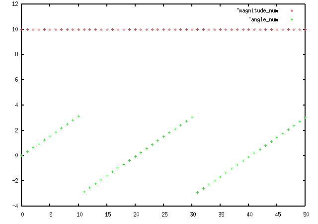
and here is the output:

as you can see the magnitude stays a steady 10, while the angle continuously runs from zero to pi (3.14159), then -pi to zero, etc.

Example:
This uses the same sin wave sent to complex_to_float(), the output of port 0 is sent to a disk file named "imag", and port 1 to a file named "real".

	sampling_freq = 8e6
	fg = gr.flow_graph ()

	src0 = gr.sig_source_c ( sampling_freq, gr.GR_SIN_WAVE, 396.15e3, 10, 0)

	c2f = gr.complex_to_float ()

	dst1 = gr.file_sink (gr.sizeof_float, "imag")
	dst2 = gr.file_sink (gr.sizeof_float, "real")

	fg.connect ( src0, c2f )
	fg.connect ( (c2f, 0), dst1 )
	fg.connect ( (c2f, 1), dst2 )

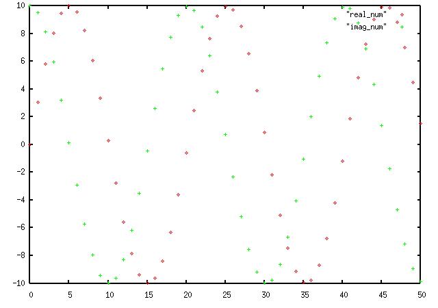
while creates this output:

where you can see real, the red dots, is indeed a sine and imaginary a cosine.

Our final example uses float_to_mag() on the AM signal we created on this page which modulated a 455Khz signal with a 1Khz tone. The following reads a file of short signed integers called "dummy.dat", runs them through a frequency translating finite impulse response low pass filter, then to our complex_to_float() module, and writes the resulting data to a disk file called "output", which is plotted after the code.

	sampling_freq = 8e6
	cfir_decimation = 250

	fg = gr.flow_graph()

	src0 = gr.file_source (gr.sizeof_short, "dummy.dat") # don't repeat

	# computer FIR filter taps
	channel_coeffs = \
		gr.firdes.low_pass (
		  1.0,		# gain
		  sampling_freq,
		  10e3,		# low pass cutoff
		  20e3,		# width of transition band
		  gr.firdes.WIN_HAMMING )

	# input: short; output: complex
	chan_filter1 = \
		gr.freq_xlating_fir_filter_scf (
		  cfir_decimation,	# reduce sampling rate to audio speed
					# 8e6 / 250 = 32,000
		  channel_coeffs,
		  455e3,		# AM carrier frequency
		  sampling_freq )

	am_demod = gr.complex_to_mag ()

	dst = gr.file_sink (gr.sizeof_float, "output")

	fg.connect ( src0, chan_filter1 )
	fg.connect ( chan_filter1, am_demod )
	fg.connect ( am_demod, dst)

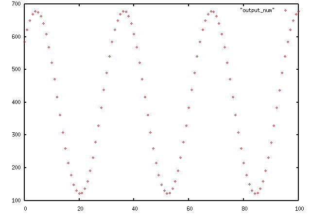
Here you can see we have recovered the 1Khz signal (32 dots every cycle at 32Khz sample rate) with a DC component from the carrier.