Experiment #3: parallel LC tank circuit
This verification experiment uses the 1nF capacitor and the 1.5uH
inductor connected in parallel
to the VNA on a breadboard and the 6" piece of RG-174.
I use the same calibration data files from experiment #1.
Then I run f_sweep_tr.py stopping at 10Mhz since they are known
to be "interesting" around 4MHz.
This creates a data file LC_parallel_refl_raw. This is compensated with
$ ./refl_calc_1.py calib_refl_open calib_refl_short calib_refl_load LC_parallel_refl_raw LC_parallel_refl_comp
and then display the results with the updated version of display_smith_data2.py
The displays:
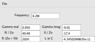
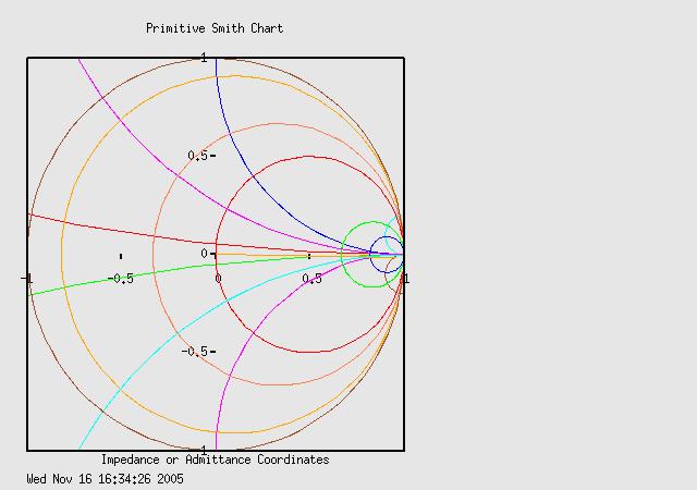
A parallel resonant tank appears as a high impedance where inductive reactance
equals capacitive reactance. Above we can see the Smith chart point toward
the infinity point, and the two components look like a 43pf cap (880 ohms
reactance) and 2K ohm resistor. In theory a 1.5uH and 1nF tank would resonate
at 4.109MHz. f = 1 / ( 2 * π * sqrt( L * C ))
Exp. 3a - This variation shows the power of calibration. I run the same test
as above, but with a 50ft piece of RG-58 between the directional coupler
and the device under test. With just the 50ft coax, I collect data for SHORT,
OPEN and with a 50 ohm LOAD. This is how the SHORT data plot looks, clearly
showing the phase shift of the endpoint impedance as the electrical length
of the cable changes with frequency:
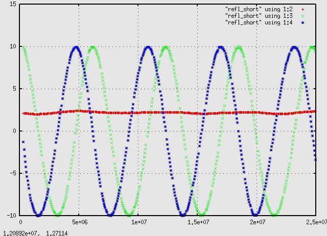
As an aside - the above shows four full rotations of the short. Keep in mind
that the directional coupler inverts the phase, and that RG-58 has a velocity
factor of about 0.66: At very low frequencies the short appears as in phase, +10
(again it's really 180 deg OUT but for the coupler), and as the cable
reaches 1/4 wavelength at 3Mhz it has been rotated around 180 deg to an open. At 2/4
wave it's back to a short at about 6Mhz, then it looks like an open again at 3/4
wave at 9Mhz and back to a short at 4/4 wave about 12Mhz. My calculations
show a full wave on 50ft of RG-58 (with velocity factor .66) would be at 12.9Mhz. The rotation
continues for another cycle (5/4, 6/4, 7/4 and 8/4 wave) up to 25Mhz, where there are two full waves,
or 4 standing waves, on the coax.
Next I connect the parallel LC tank circuit and collect the raw data, which
looks like this:
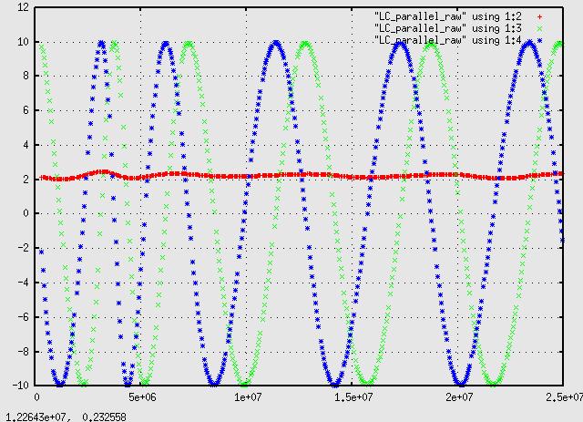
Then I process the raw data with the calibration data using
$ ./refl_calc_1.py refl_open refl_short refl_load LC_parallel_raw LC_parallel_comp
and when the compensated data is plotted I get this:
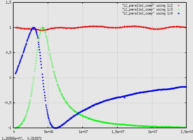
where the effects of the 50ft piece of RG-58 have been magically removed, and
clearly showing the in-phase (green curve) high impedance point right around 4.2MHz.