Transmission/Reflection Vector Network Analyzer
with calibration and compensation
Support Docs: McDermott TAPR VNA Article
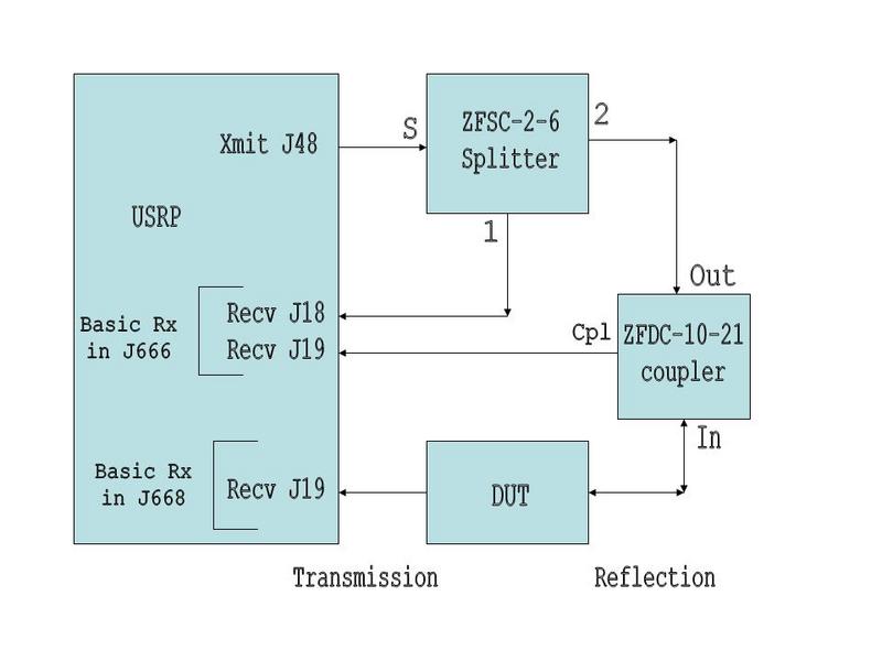
Hardware setup:
(Nov. 15, 2005) Finally added calibration and compensation routines to the magnitude
and phase measuring scripts. Instead of trying to make one complete
do-it-all application I've broken the tasks down into a set of
individual scripts that collect data, process it, and format and
display data.
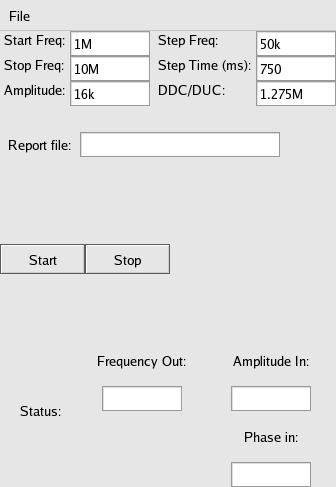
- f_sweep_tr2.py
Data collection script.
Frequency Sweeper outputs a signal in a frequency range (for example, 250kHz
to 25MHz) and records transmission or reflection magnitude and phase to a
disk file. Select transmission port or reflection port with command line
options which sets the apropriate mux. Default is reflection.
- trans_calc_1.py
Processing script.
Takes as input a transmission calibration file, a test device data file
and produces compensated output. Requires 3 command line file specifications.
- refl_calc_1.py
Processing script.
Takes as input 3 calibration files: open, short and load; a test device
data file and output file for the compensated data. Processed (calibration
compensated) data can be plotted with gnuplot to show magnitude, but phase
is difficult to interpret.
- convert_rpt_to_smith3.py
will convert any of the above files (in format: freq mag phase sphase) into
a rectangular form (format: freq x y) suitable for plotting with gnuplot
using smith_chart.
- display_smith_data.py
will
display the 'rpt' format (freq mag phase sphase) files in a neat chart
with Powermate knob control of frequency. That is, you can scroll up and
down in freq and see the point on the smith chart move about while reading
the frequency off a window.
f_sweep_tr2.py:
Transmission Measurements
Calibration for transmission measurements is
pretty easy. With the test jig wired, we put a 'bullet' or short
through-connect in place of the device to test, then run a freq scan with
f_sweep_tr2.py and save the data to a calibration
file for later use. Then we remove the 'bullet' and connect the test
device, a filter or what have you, in it's place and run another scan and
save the data to a device data file. Once we have those two, calculating
the actual transmission response is easy. The theory is:
s21(actual) = s21(measured) / CAL21 (See McDermott)
s21(actual), (measured) and CAL21 are all complex mag/phase values collected
for each frequency with f_sweep_tr2.py. trans_calc_1.py is the script that
applies the calibration compensation to the data. Say we have run f_sweep_tr2.py
with a connect-through 'bullet' and collected data into a file "calib_trans".
Then removed the bullet and connected a device, ran f_sweep_tr2.py and
collected data into a file "dut_data_raw". We can then apply compensation with:
$ ./trans_calc_1.py calib_trans dut_data_raw dut_data_comp
Once the compensated data is obtained, you can display it on a static
Smith chart by converting it to rectangular form:
$ ./convert_rpt_to_smith3.py dut_data_comp dut_data_comp_smith
and putting the file name in smith_chart and
displaying with:
$ gnuplot smith_chart
OR displaying it on a dynamic Smith chart with Powermate knob control:
$ ./display_smith_data.py dut_data_comp
Reflection Measurements
Reflection is a bit more involved as we need to make 3 calibration data files,
one with the DUT disconnected (open), one with a short for the DUT (short),
and one with a 50ohm load resistor for a DUT (load). Once we have created
those three files with f_sweep_tr2.py, we can connect the test DUT and collect
the test device data. Once we have the test device data and the calibration
data we apply compensation with:
$ ./refl_calc_1.py calib_open calib_short calib_load dut_data_raw dut_data_comp
and then plot or display it as above. The compensation math is more complicated
and I refer you to McDermott above for all the gory details.
Examples
Transmission test: This just shows that "Anything / Anything = 1" where
Anything does not equal zero, and demonstrates that transmission calibration
actually works. With a through-connect 'bullet' in place we run f_sweep_tr2.py (remembering to start it with a -tt command line option)
from 250kHz to 25MHz and save the data to "calib_trans". Then I run it again
(testing repeatability) and save the data to "calib_trans_2". Then I use the
first file as calibration data, the second file as device data and plot the
results. Here is a plot of the calibration data:
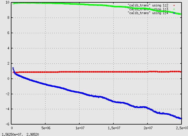
and of course the test data, "calib_trans_2" looks very similar. After
processing:
$ ./trans_calc_1.py calib_trans calib_trans_2 test_data
and when the conpensated 'bullet' test data is plotted:
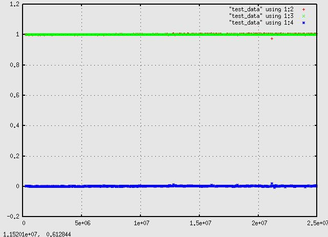
which shows phase and magnitude at unity across the spectrum from 250kHz to
25MHz. Next we connect an actual device, my 80mtr ham bandpass filter,
run f_sweep_tr2.py and save the collected data as "80mtr_pass-filter_raw_data",
then process it:
$ ./trans_calc_1.py calib_trans 80mtr_pass-filter_raw_data 80mtr_pass-filter_comp_data
which, when plotted:
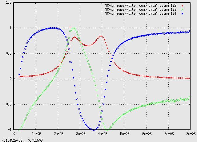
which looks somewhat like the uncompensated plot but the slow 90 degree
or so phase shift error over a 25MHz scan has been magically removed!
Next we try a similar process with reflected measurements. First run f_sweep_tr2.py
and get data for open (calib_refl_open), short (calib_refl_short) and with a
50ohm load (calib_refl_load). This is how the calib_refl_short data looks:
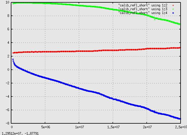
again with the slow phase shift. When we run conpensation on the "short" file:
$ ./refl_calc_1.py calib_refl_open calib_refl_short calib_refl_load calib_refl_short calib_refl_short_comp
it turns out like this:
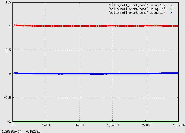
showing a nice even magnitude of 1 and a phase of -1 (180deg) across the
spectrum. Finally, plugging in the filter, repeat the above, we get
this plot of it's reflection characteristics:
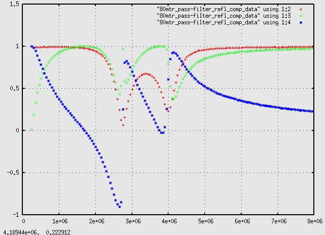
We can convert the polar data (in "freq mag phase sphase" format) to
rectangular:
$ ./convert_rpt_to_smith3.py 80mtr_pass-filter_refl_comp_data 80mtr_pass-filter_refl_comp_data_smith
and plugging "80mtr_pass-filter_refl_comp_data_smith" into smith_chart
and running
$ gnuplot smith_chart
it comes out:
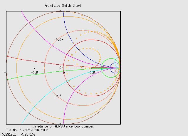
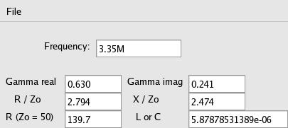
and even more fun is to load the polar data
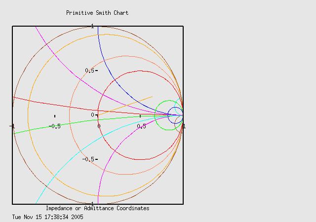
into display_smith_data2.py and play with the Powermate knob. With the
knob adjusted to the outside of the middle lobe (corresponding to the
middle of the 'saddle' in the above plot) it looks like:
Notes: The calibration files and the device data files MUST match in frequency.
The calibration files must start at the same frequency and include the entire range in the
device data file. That is, if the device data is collected from 5 to 15MHz,
the calibration files MUST also start at 5MHz and go up to at least 15MHz,
altho it can go higher (as soon as device data runs out compensation processing
stops). If the frequencies do not match up you will get an error message.