Magnitude and Phase measurement, Part II
This is one of the first working plots of the magnitude and phase response
of a 2.5 to 4.2Mhz filter over a wide frequency range:
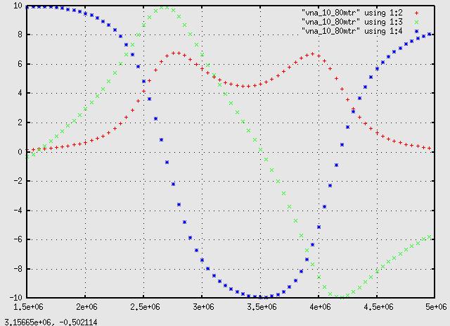
Red is the amplitude response, and green the phase response. +10 is "in phase"
or 0 degree, and -10 is π (180deg) out of phase. Since the phase
meter is measuring the cosine of an angle, the sign of the phase is ambiguous.
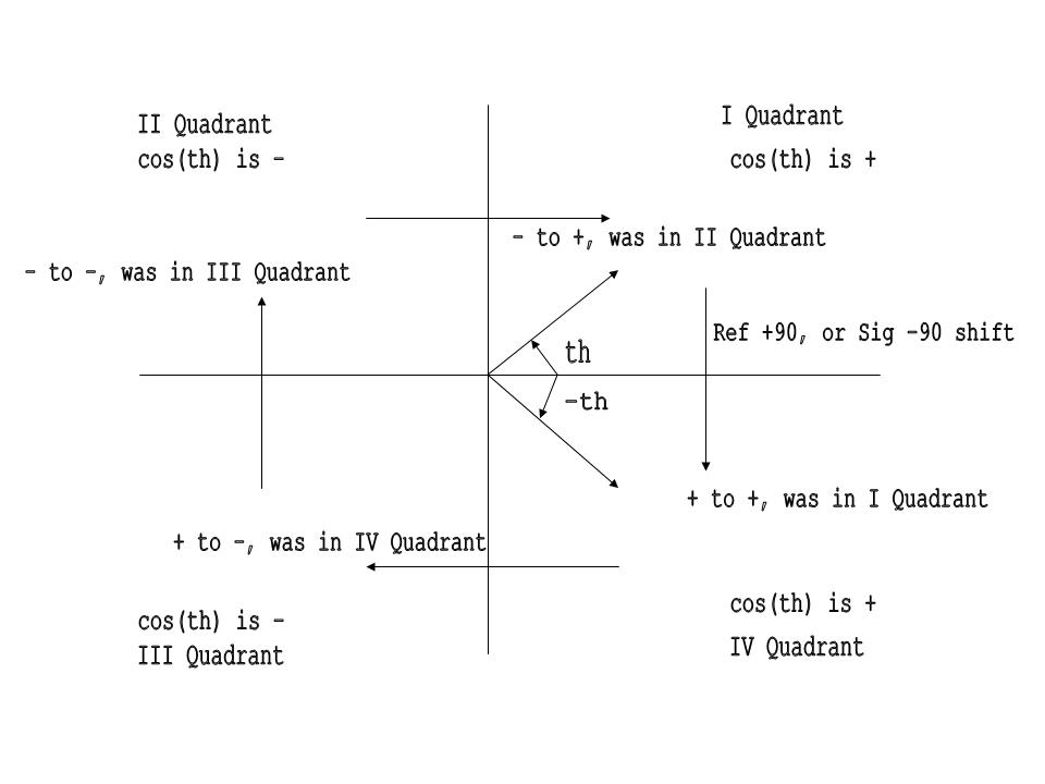
That is, cos(th) = cos(-th). To resolve this, we introduce a π/2 (90deg)
phase advance in the reference signal (equivilent to a π/2 delay in the
measured signal). If the sign is + and remains + after advancing the reference
signal, the difference phase angle is in the 1st (I) quadrant, or 0 to π/2.
This is equivilent to delaying the measured signal, or rotating it clockwise, by 90 deg.
If the sign is - and remains - it is in the 3rd (III) quadrant or -&pi/2 to -π.
If the sign is + and changes to - it is in the 4th (IV) quadrant, 0 to -π/2,
and if it is - and changes to + it is in the 2nd (II) quadrant, or π/2 to π.
In the plot above the phase starts out at 1.5Mhz with about 90 degrees out of
phase and shifts with rising frequency toward 0 degrees or in phase at about
2.7Mhz. At that point the sign of the shifted-reference phase measurement
(blue) changes so the phase has moved clockwise around from the 1st to the
4th quadrant, continuing on untill the phase is -180 degrees at about 4.2Mhz
and then on around clockwise into the 2nd quadrant trending back to 90 degrees.
This is the spice plot:
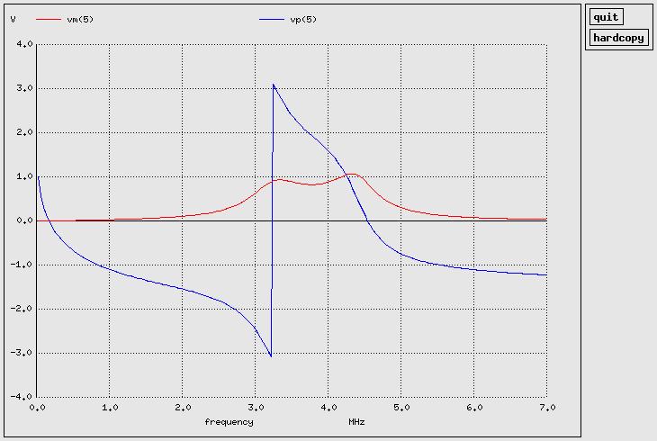
The real filter in the top plot has the passband about 300khz too low (due to
real component values I guess) but the important thing here is the relationship
of the phase to the amplitude response. And for some reason the spice plot
is just the opposite, with π phase shift at 3.2Mhz and 0 at 4.5Mhz.
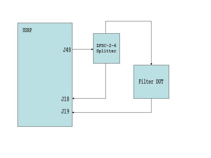
Shortly I hope to have a test jig and software to measure both reflected
and transmitted response of two port networks, or just reflected resonse
of single port networks (like an antenna). Measuring reflected & transmitted
signal will require two basic input boards for 3 inputs including the reference
signal from the splitter.
This is the test jig:
The code so far:
f_sweep_2a.py
(recent version no longer needs custom blocks for measuring signal levels in python)
Nov 10, 2005: Fixed a bug where I had magnitude squared instead of magnitude:
io_ratio = math.sqrt((out_level / in_level)) # scaled to match phase plot
since the output of gr.signal_level_cc() is the square of the peak signal value.
The code uses a sampling rate of 1Mhz for the transmit and 2 receiver channels.
That limits the sweep width to a max of -500 to 500Khz, realistically -275 to
275Khz. I chose 11 samples 50Khz apart over a -275 to 275Khz range so that
they will straddle the 0Hz center, there will be a sample at -25Khz, then the
next at 25Khz, staying comfortably out of the range where the phase meter
cannot filter out the 2X frequency. After sweeping 550Khz like that, the code
must stop the timer, stop the signal generator graph and delete it, stop the
receiver graph, stop the DDC's, change the receiver DDC center
frequency, rebuild the generator at a new DUC freq, start the generator, start
the receiver, and restart the timer. There are a few time delays to allow for
settling. It gets 1 data point every 750mSec, with a longer delay when changing
DUC/DDC frequency.
This is a polar plot of the above data:

I have NO idea what, if anything, it means but thought it looked pretty
and serves as a test of getting data into normalized rectangular form
with a Smith Chart background. More about that coming soon.
The left, lower freq hump in the earlier plot corresponds to the right
lobe of this one. The pattern is the same - at low f the phase is near +90,
rotates around to 0 deg in phase near the top of the first hump, then
swings around down clockwise to near -90 in the middle between the humps
then around clockwise to near -180 after the higher freq hump and then
back towards +90 while decreasing in magnitude. That is, from low to
high freq the points go clockwise around the curve.
The Smith Chart for GNUPlot, modified thus:
set size square
set time
set clip
set xtics axis nomirror
set ytics axis nomirror
unset grid
unset polar
set title "Primitive Smith Chart"
unset key
set xlabel "Impedance or Admittance Coordinates"
set para
set rrange [-0 : 10]
set trange [-pi : pi]
set xrange [-1:1]
set yrange [-1:1]
tv(t,r) = sin(t)/(1+r)
tu(t,r) = (cos(t) +r)/(1+r)
cu(t,x) = 1 + cos(t)/x
cv(t,x) = (1+ sin(t))/x
plot cu(t,.1),cv(t,.1),cu(t,.1),-cv(t,.1),\
cu(t,1),cv(t,1),cu(t,1),-cv(t,1),\
cu(t,10),cv(t,10),cu(t,10),-cv(t,10),\
tu(t,.1),tv(t,.1),\
tu(t,.5),tv(t,.5),\
tu(t,1),tv(t,1),\
tu(t,5),tv(t,5),\
tu(t,10),tv(t,10),\
cu(t,.5),cv(t,.5),cu(t,.5),-cv(t,.5),\
tu(t,0),tv(t,0), "YOUR_DATA_HERE"
pause -1
where YOUR_DATA_HERE is a text file in your current directory with two
column XY data in the range -1 to 1.
Modification to the report writing code to make polar plots:
              if self.rpt_open == True:
              #  self.rpt.write(str(freq)+" "+str(io_ratio)+" "+str(phase)+" "+str(sphase)+"\n")
              # output for smith chart. Convert magnitude and angle into rect
              # coords -1 to 1
                if ((phase > 0) & (sphase > 0)) | ((phase < 0) & (sphase > 0)) :                  # 1st or 2nd quad
                  ang = math.acos(phase/10)
                if ((phase > 0) & (sphase < 0)) | ((phase < 0) & (sphase < 0)) :                  # 4th or 3rd quad
                  ang = -math.acos(phase/10)
                x_pos = math.cos(ang) * io_ratio/10
                y_pos = math.sin(ang) * io_ratio/10
                self.rpt.write(str(x_pos)+"  "+str(y_pos)+"\n")